Problem Description
An animated simulation of three varieties of
pendulum: Simple, Double, and Forced.
Background & Techniques
I recently implemented a Delphi version of the Runge-Kutta technique for
solving second order ordinary differential equations. This type
of equation is good at describing the motion of things ( the second order
part translates to acceleration) so sliding, rolling, bouncing, vibrating,
rotating, swinging
things are all candidates. I chose swinging for this program and
learned some interesting things about pendulums. The following "User
guide" is also available in the program buy clicking the Info buttons
in the program.
Introduction
This program
explores three different types of pendulums. Each of the
following pages allows the user to set parameters defining the pendulums
and set them in motion to observe the effect. The program was
written to test a recently developed Runge-Kutta technique for solving a
single ordinary differential equation (ODE) or a system of ODEs.
If you are not into higher mathematics or programming, it’s still fun to
play with the parameters and observe results. The dual double
pendulums and the forced damped pendulums make interesting viewing.
Simple Pendulum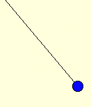
A Simple Pendulum
consists of a weight or “bob” hanging freely from the end of a weightless
rod of length L. Rotating the bob to some initial angle,
q0,
and releasing it imparts its movement. Gravity, G,
pulls the bob in a downward arc and past vertical to angle equal to the
initial displacement, unless some damping force slows it down.
Damping factor, D, is a constant which when multiplied by the
angular velocity, q',
produces a force acting to decrease the velocity.
The differential equation is:
q'' =
- G/L sin (q) – Dq'
In words, the acceleration of the bob is equal
to that part of the gravitational force acting perpendicular to the
shaft minus the damping force. The minus sign on the gravity
term just tells us that gravity is the enemy here, always trying to slow
things down.
Our Runge-Kutta procedure calls a user-defined
function, passing an angle (q) and angular velocity (q') for each time interval. The function in this
case applies the above equation to return a new angular acceleration value
(q'').
Here’s the Delphi code:
Function
TForm1.Pendulum1Func(T, X, Xprime: Float):Float;
begin
Result: = - Gravity/Len*sin(x) – Damping * Xprime;
end;
The simple pendulum program page lets you to
change gravity, length, initial angle and damping factor and
watch the pendulum run.
The Computational Parameters
dialog allows setting maximum run time, calculated points per second (pps)
and returned pps. The default values, 100 pps calculated and
25 pps returned usually provide reasonably accurate values and smooth
plots. Points returned should be some fraction of points
calculated per second, normally returning around 25% of the calculated
samples will work fine for the display.
By the way, it is often supposed that
the period of a pendulum (the time to make a complete swing), is
independent of length, mass, or swing angle. This is almost true.
The pendulum does swing faster at smaller angles as you can check
for yourself by setting the damping factor to 0 and timing 10 swings for
various starting angles.
Note: All angles are measured counterclockwise
from South (down).
Double Pendulums
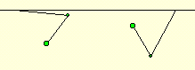
The second pendulum page
has one pendulum attached to the end of another pendulum, like holding a
weight in your hand and swinging it with your shoulder and a really flexible elbow. Do a web search on “double pendulum” and you
will find a number of sites that list the differential equations.
Unlike a simple pendulum, the equations for double pendulums do include
the masses of the bobs.
Here we test our Runge-Kutta procedure’s
ability to solve a system of differential equations. There are
separate ODEs for each part of the pendulum and they interact, i.e. the
acceleration of each bob is influenced by the acceleration of the other.
The ODEs are quite complex so I won’t bother to reproduce them here.
They are available on-line or in the source code for this program for
those interested.
This page
includes a “chaos” demonstration; a very small change resulting in very
different behavior. In this “dual double pendulum “example, we’ll
clone the defined pendulum, multiply the mass of the lower bob by 1.0001
on the clone, and then release them at the same time. After a minute
or two the behaviors will diverge and have no apparent relationship to
each other. A search on the web for “butterfly effect”
will produce some interesting reading about this sensitivity to initial
conditions.
Forced Pendulum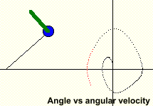
The final page let’s you play with a
Damped Forced Pendulum. In this case, a force of specified
amplitude, A, and frequency, Ω (omega), is applied to a
simple pendulum. The equation is often simplified by assuming
pendulum length is equal to the value for gravity since the interesting
effects involve damping factor, D, and the characteristics of the
forcing frequency at time t. I’ve chosen to leave
gravity, G, and length, L, in the calculations.
q''
= – Dq' - G/L sin(q)
+ Asin(Ωt)
Or,
in Delphi terms:
Function
TForm1.Pend3Func(T, X, XPrime: Float): Float;
begin
Result: = - Damping* Xprime – Gravity/Length*sin (X) +
A* cos(omega*T);
end;
The pendulum animation displays the
applied force as a green bar acting on the bob at right angles to the
pendulum and with length proportional to the value of the force.
A separate chart plotting pendulum angle
vs. angular velocity is also displayed. It may take the
pendulum a minute or more to stabilize due to damping effects as it starts
from the resting position. Clicking the “Clear chart” button
after a couple of minutes will give a clearer impression of the steady
state pattern,( if there is one). There is also a
“Real time” checkbox that toggles the display between real time and
the maximum display rate for your computer and graphics card.
An appropriate
selection of input values will produce patterns that repeat in single,
double loops or chaotic behavior that may never repeat.
Starting with the default values, try runs with amplitudes from 100 to 120
to see a variety of interesting behaviors.
Non-programmers are welcome to read on, but may
want to skip to the bottom of this page to download
executable version of the program.
Programmer Notes
The length of this program puts it in the Advanced category, but there
were no great programming challenges once you understand the calling
protocol for Runge-Kutta described on this
Runge-Kutta page over in the Math
Topics section.
There are a couple of other new (at least for me) items worth
mentioning: